3.8. Plotting
This notebook demonstrates some of Conx’s functions for visualizing the behavior of networks. First, let’s create a simple XOR network to explore.
In [1]:
import conx as cx
Using TensorFlow backend.
Conx, version 3.6.1
In [2]:
net = cx.Network("XOR 2-3-1 Network")
net.add(cx.Layer("input", shape=2))
net.add(cx.Layer("hidden", shape=3, activation='sigmoid'))
net.add(cx.Layer("output", shape=1, activation='sigmoid'))
net.connect()

XOR = [
    ([0, 0], [0], "1"),
    ([0, 1], [1], "2"),
    ([1, 0], [1], "3"),
    ([1, 1], [0], "4")
]
net.dataset.load(XOR)
net.dataset.info()

net.compile(loss='mean_squared_error', optimizer='sgd', lr=0.3, momentum=0.9)
Dataset: Dataset for XOR 2-3-1 Network
Information: * name : None * length : 4
Input Summary: * shape : (2,) * range : (0.0, 1.0)
Target Summary: * shape : (1,) * range : (0.0, 1.0)
In [3]:
net.picture()
Out[3]:
In [4]:
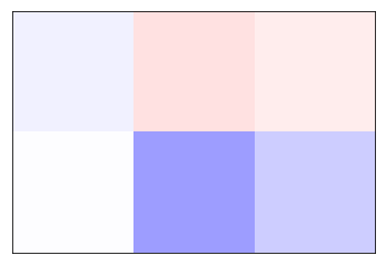
cx.view(net.get_weights_as_image("hidden"))
In [8]:
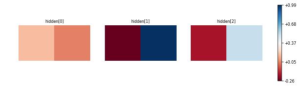
net.plot_layer_weights('hidden', colormap="RdBu"
In [6]:
net.train(epochs=1000, accuracy=1, report_rate=25, record=True)

========================================================
       |  Training |  Training
Epochs |     Error |  Accuracy
------ | --------- | ---------
#  533 |   0.00652 |   1.00000
In [7]:
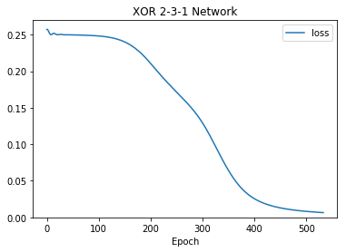
net.plot('loss', ymin=0)
3.8.1. plot_activation_map
This plotting function allows us to see the activation of a specific unit in a specific layer, as a function of the activations of two other units from an earlier layer. In this example, we show the behavior of the single output unit as the two input units are varied across the range 0.0 to 1.0:
In [8]:
net.plot_activation_map('input', (0,1), 'output', 0)
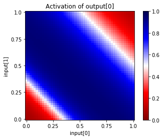
We can verify the above output activation map by running different input vectors through the network manually:
In [9]:
print(net.propagate([0,0])[0])
print(net.propagate([1,1])[0])
print(net.propagate([0.5, 0.5])[0])
print(net.propagate([0, 0.6])[0])
0.06735210865736008
0.09960916638374329
0.9248424768447876
0.8984166383743286
In [10]:
# map of hidden[2] activation as a function of the inputs
net.plot_activation_map('input', (0,1), 'hidden', 2, show_values=True)
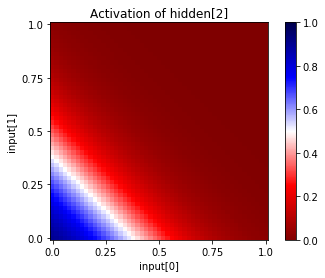
----------------------------------------------------------------------------------------------------
Activation of hidden[2] as a function of input[0] and input[1]
rows: input[1] decreasing from 1.00 to 0.00
cols: input[0] increasing from 0.00 to 1.00

0.03 0.02 0.01 0.01 0.01 0.01 0.00 0.00 0.00 0.00 0.00 0.00 0.00 0.00 0.00 0.00 0.00 0.00 0.00 0.00
0.04 0.03 0.02 0.01 0.01 0.01 0.01 0.00 0.00 0.00 0.00 0.00 0.00 0.00 0.00 0.00 0.00 0.00 0.00 0.00
0.05 0.04 0.03 0.02 0.01 0.01 0.01 0.01 0.00 0.00 0.00 0.00 0.00 0.00 0.00 0.00 0.00 0.00 0.00 0.00
0.06 0.05 0.04 0.03 0.02 0.01 0.01 0.01 0.01 0.00 0.00 0.00 0.00 0.00 0.00 0.00 0.00 0.00 0.00 0.00
0.09 0.06 0.05 0.04 0.03 0.02 0.01 0.01 0.01 0.01 0.00 0.00 0.00 0.00 0.00 0.00 0.00 0.00 0.00 0.00
0.11 0.09 0.06 0.05 0.04 0.03 0.02 0.01 0.01 0.01 0.01 0.00 0.00 0.00 0.00 0.00 0.00 0.00 0.00 0.00
0.15 0.11 0.08 0.06 0.05 0.04 0.03 0.02 0.01 0.01 0.01 0.01 0.00 0.00 0.00 0.00 0.00 0.00 0.00 0.00
0.19 0.15 0.11 0.08 0.06 0.05 0.04 0.03 0.02 0.01 0.01 0.01 0.01 0.00 0.00 0.00 0.00 0.00 0.00 0.00
0.24 0.19 0.15 0.11 0.08 0.06 0.05 0.03 0.03 0.02 0.01 0.01 0.01 0.01 0.00 0.00 0.00 0.00 0.00 0.00
0.30 0.24 0.19 0.15 0.11 0.08 0.06 0.05 0.03 0.03 0.02 0.01 0.01 0.01 0.01 0.00 0.00 0.00 0.00 0.00
0.37 0.30 0.24 0.19 0.14 0.11 0.08 0.06 0.05 0.03 0.03 0.02 0.01 0.01 0.01 0.01 0.00 0.00 0.00 0.00
0.44 0.37 0.30 0.24 0.19 0.14 0.11 0.08 0.06 0.05 0.03 0.03 0.02 0.01 0.01 0.01 0.01 0.00 0.00 0.00
0.52 0.44 0.37 0.30 0.24 0.19 0.14 0.11 0.08 0.06 0.05 0.03 0.03 0.02 0.01 0.01 0.01 0.01 0.00 0.00
0.59 0.52 0.44 0.37 0.30 0.24 0.19 0.14 0.11 0.08 0.06 0.05 0.03 0.03 0.02 0.01 0.01 0.01 0.01 0.00
0.67 0.59 0.52 0.44 0.37 0.30 0.24 0.18 0.14 0.11 0.08 0.06 0.05 0.03 0.03 0.02 0.01 0.01 0.01 0.01
0.73 0.67 0.59 0.52 0.44 0.36 0.30 0.24 0.18 0.14 0.11 0.08 0.06 0.05 0.03 0.03 0.02 0.01 0.01 0.01
0.79 0.73 0.66 0.59 0.52 0.44 0.36 0.30 0.23 0.18 0.14 0.11 0.08 0.06 0.05 0.03 0.02 0.02 0.01 0.01
0.83 0.79 0.73 0.66 0.59 0.51 0.44 0.36 0.29 0.23 0.18 0.14 0.11 0.08 0.06 0.05 0.03 0.02 0.02 0.01
0.87 0.83 0.78 0.73 0.66 0.59 0.51 0.44 0.36 0.29 0.23 0.18 0.14 0.11 0.08 0.06 0.05 0.03 0.02 0.02
0.90 0.87 0.83 0.78 0.73 0.66 0.59 0.51 0.43 0.36 0.29 0.23 0.18 0.14 0.11 0.08 0.06 0.04 0.03 0.02
----------------------------------------------------------------------------------------------------
In [11]:
# map of output activation as a function of hidden units 1,2
net.plot_activation_map('hidden', (1,2), 'output', 0)
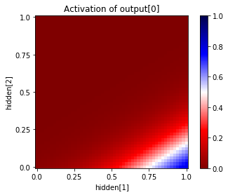
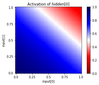
How does the network actually solve the problem? We can look at the intermediary values at the hidden layer by plotting each of the 4 hidden units in this manner:
In [12]:
net.plot_activation_map('input', (0,1), 'hidden', 0)
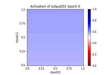
In [13]:
net.playback(lambda net,epoch: net.plot_activation_map(title="Epoch %s" % epoch, format='image'))
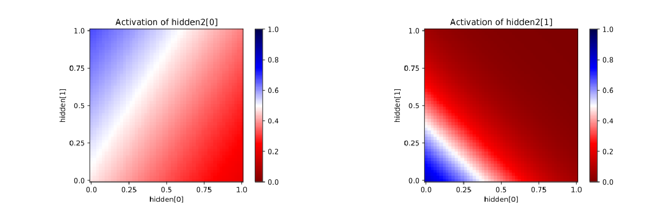
3.8.2. Adding Additional Hidden Layers
In [14]:
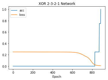
net = cx.Network("XOR 2-3-2-1 Network")
net.add(cx.Layer("input", shape=2))
net.add(cx.Layer("hidden", shape=3, activation='sigmoid'))
net.add(cx.Layer("hidden2", shape=2, activation='sigmoid'))
net.add(cx.Layer("output", shape=1, activation='sigmoid'))
net.connect()

XOR = [
    ([0, 0], [0], "1"),
    ([0, 1], [1], "2"),
    ([1, 0], [1], "3"),
    ([1, 1], [0], "4")
]
net.compile(loss='mean_squared_error', optimizer='sgd', lr=0.3, momentum=0.9)
net.dataset.load(XOR)
In [15]:
net.reset()
net.train(epochs=2000, accuracy=1, report_rate=25)

========================================================
       |  Training |  Training
Epochs |     Error |  Accuracy
------ | --------- | ---------
#  886 |   0.00721 |   1.00000
In [16]:
#net.plot_activation_map('hidden', (0,1), 'hidden2', 1)
cx.view([net.plot_activation_map('hidden', (0,1), 'hidden2', i, format='svg') for i in range(2)], scale=10)
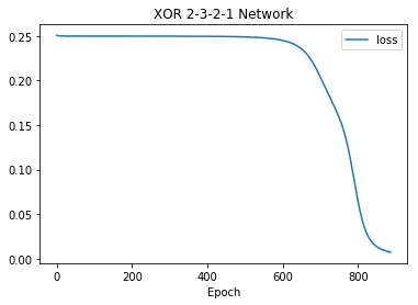
3.8.3. Plotting training error (loss) and training accuracy (acc)
In [17]:
net.plot("loss")
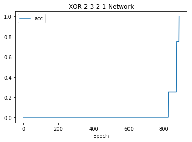
In [18]:
net.plot("acc")
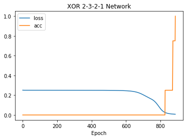
In [19]:
net.plot(["loss", "acc"])
In [20]:
net.plot("all")
3.8.4. Plotting Your Own Data
In [21]:
data = ["Type 1", [(0, 1), (1, 2), (2, .5)]]
cx.scatter(data)
Out[21]:

In [22]:
data = ["My Data", [1, 2, 6, 3, 4, 1]]
symbols = {"My Data": "rx"}
cx.plot(data, symbols=symbols)
Out[22]:

In [23]:
data = [["My Data", [1, 2, 6, 3, 4, 1]],
        ["Your Data", [2, 4, 5, 1, 2, 6]]]
symbols = {"My Data": "rx-", "Your Data": "bo-"}
cx.plot(data, symbols=symbols)
Out[23]:
