3.3. The MNIST Dataset

In this notebook, we will create a neural network to recognize handwritten digits from the famous MNIST dataset.

We will experiment with two different networks for this task. The first one will be a multi-layer perceptron (MLP), which is a standard type of feedforward neural network with fully-connected layers of weights, and the second will be a convolutional neural network (CNN), which takes advantage of the inherently two-dimensional spatial geometry of the input images.

Let’s begin by reading in the MNIST dataset and printing a short description of its contents.

import conx as cx
mnist = cx.Dataset.get('MNIST')
mnist.info()

Dataset: MNIST

Original source: http://yann.lecun.com/exdb/mnist/

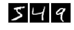
The MNIST dataset contains 70,000 images of handwritten digits (zero to nine) that have been size-normalized and centered in a square grid of pixels. Each image is a 28 × 28 × 1 array of floating-point numbers representing grayscale intensities ranging from 0 (black) to 1 (white). The target data consists of one-hot binary vectors of size 10, corresponding to the digit classification categories zero through nine. Some example MNIST images are shown below:

MNIST Images

Information: * name : MNIST * length : 70000

Input Summary: * shape : (28, 28, 1) * range : (0.0, 1.0)

Target Summary: * shape : (10,) * range : (0.0, 1.0)

We will split the 70,000 digits into a training set of 60,000 images and a testing set of 10,000 images.

mnist.split(10000)
mnist.summary()

_________________________________________________________________
MNIST:
Patterns    Shape                 Range
=================================================================
inputs      (28, 28, 1)           (0.0, 1.0)
targets     (10,)                 (0.0, 1.0)
=================================================================
Total patterns: 70000
   Training patterns: 60000
   Testing patterns: 10000
_________________________________________________________________

The training and testing images can be referenced independently, via the dataset properties train_inputs and test_inputs. The inputs property refers to all 70,000 input images.

print(len(mnist.inputs), 'total images')
print(len(mnist.train_inputs), 'images for training')
print(len(mnist.test_inputs), 'images for testing')

70000 total images
60000 images for training
10000 images for testing

Let’s take a look at some individual input images.

cx.view(mnist.train_inputs[0])  # same as mnist.inputs[0]

cx.view(mnist.train_inputs[0:5])   # same as mnist.inputs[0:5]

cx.view(mnist.train_inputs[0, 2, 4])

selected = [42, 77, 150, 16, 15, 0]
cx.view(mnist.train_inputs[selected])

cx.view(mnist.test_inputs[0])

cx.view(mnist.test_inputs[0:5])

The dataset properties train_targets, train_labels, test_targets, and test_labels refer to the target data.

mnist.test_labels[0:5]

['7', '2', '1', '0', '4']

mnist.test_targets[0:5]

[[0.0, 0.0, 0.0, 0.0, 0.0, 0.0, 0.0, 1.0, 0.0, 0.0],
 [0.0, 0.0, 1.0, 0.0, 0.0, 0.0, 0.0, 0.0, 0.0, 0.0],
 [0.0, 1.0, 0.0, 0.0, 0.0, 0.0, 0.0, 0.0, 0.0, 0.0],
 [1.0, 0.0, 0.0, 0.0, 0.0, 0.0, 0.0, 0.0, 0.0, 0.0],
 [0.0, 0.0, 0.0, 0.0, 1.0, 0.0, 0.0, 0.0, 0.0, 0.0]]

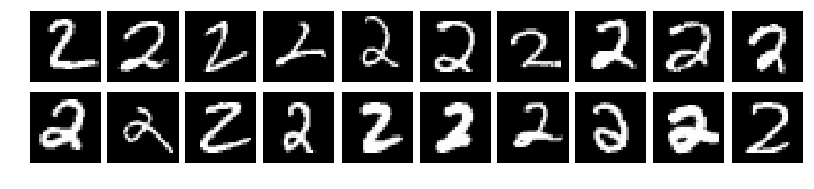
As another example, we could use test_labels to select digits of a particular category from the testing data, and then view the first twenty, as follows:

selected = [i for i in range(len(mnist.test_inputs)) if mnist.test_labels[i] == '2']
digits = mnist.test_inputs[selected]
cx.view(digits[:20], layout=(2,10))

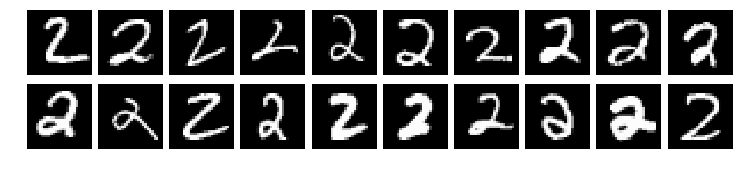
We can accomplish the same thing more directly (and efficiently) using the select method, together with the slice keyword:

digits = mnist.test_inputs.select(lambda i,ds: ds.test_labels[i] == '2', slice=20)
cx.view(digits, layout=(2,10))

The MNIST digits are grayscale images, with each pixel represented as a single intensity value in the range 0 (black) to 1 (white). You can think of the whole image as consisting of 784 numbers arranged in a plane of 28 rows and 28 columns. For color (RGB) images, however, each pixel consists of three numbers (one for Red intensity, one for Green, and one for Blue). Therefore color images are represented as arrays of shape rows × columns × 3, where the 3 indicates the depth of the image. For consistency, the grayscale MNIST images are treated as images of depth 1, with shape rows × columns × 1. We can verify this by calling cx.shape on input image #0:

cx.shape(mnist.inputs[0])

(28, 28, 1)

3.3.1. A Multi-Layer Perceptron for MNIST Classification

Our first network will have an input layer, two fully-connected hidden layers, and an output layer containing 10 output units (one for each possible digit category). Since this is a classification task, the output layer will use the Softmax function to generate a probability distribution of output values, where each value is a number in the range 0-1 representing the probability that the input image corresponds to that output unit’s digit category.

The input layer’s shape must match that of the input data, so we declare its shape to be (28,28,1). We then add two densely-connected hidden layers of 30 units each, both of which use the ReLU (rectified linear) activation function. However, we cannot connect the input layer directly to the first hidden layer, because the layer shapes do not match. Instead, we must first “flatten” the data before feeding it into the first hidden layer. Finally, we add an output layer of 10 units that uses the Softmax activation function. Here is the code that builds the network:

net = cx.Network("MNIST_MLP")

net.add(cx.Layer("input", (28,28,1)),
        cx.FlattenLayer("flat_input"),
        cx.Layer("hidden1", 30, activation='relu', dropout=0.20),
        cx.Layer("hidden2", 30, activation='relu', dropout=0.20),
        cx.Layer("output", 10, activation='softmax'))

# creates connections between layers in the order they were added
net.connect()

Notice that each hidden layer in the network includes a dropout setting of 20%. Dropout is a technique that helps to improve a network’s ability to generalize what it has learned, by making it less sensitive to noise and to irrelevant correlations that may exist in the training data. During training, a randomly chosen subset of units in a dropout layer (here, 20% of the units) will be turned off (set to zero activation) on each training cycle, with different random subsets being chosen on each cycle. Dropout only occurs during training; after the network has learned, all units participate in the classification of input data.

Finally, we need to tell the network which dataset to use.

net.set_dataset(mnist)

We are now ready to compile the network. To do so, we must specify the error (or “loss”) function that measures the network’s performance, and the specific learning algorithm for optimizing the network’s weights during training. For a classification task using Softmax, in which the output of the network is a probability distribution across several possible classification categories, the appropriate error function is usually the categorical crossentropy function. The choice of optimizer is typically some variant of stochastic gradient descent. Here we will use RMSprop. After compiling the network, it is ready to be trained. The summary() method prints out a brief summary of each layer, including the total number of trainable parameters (weights and biases) in the network.

net.compile(error='categorical_crossentropy', optimizer='rmsprop')
net.summary()

_________________________________________________________________
Layer (type)                 Output Shape              Param #
=================================================================
input (InputLayer)           (None, 28, 28, 1)         0
_________________________________________________________________
flat_input (Flatten)         (None, 784)               0
_________________________________________________________________
hidden1 (Dense)              (None, 30)                23550
_________________________________________________________________
dropout_1 (Dropout)          (None, 30)                0
_________________________________________________________________
hidden2 (Dense)              (None, 30)                930
_________________________________________________________________
dropout_2 (Dropout)          (None, 30)                0
_________________________________________________________________
output (Dense)               (None, 10)                310
=================================================================
Total params: 24,790
Trainable params: 24,790
Non-trainable params: 0
_________________________________________________________________

Let’s take a look at the network before we train it. The dashboard provides an easy-to-use graphical interface, showing the network’s response to each input image in the dataset. (The small ⦻ symbols indicate layers with dropout.)

dash = net.dashboard()
dash

Clicking on MNIST_MLP at the top of the dashboard will open up a panel of settings for controlling the appearance and functionality of the network display. For example, to choose between the training set and testing set images, you can select “Train” or “Test” from the Dataset pulldown menu.

The propagate method sends an input pattern through the network and returns a list of the output values. In the example below, the outputs are all around 0.1 because the network has not yet been trained. After training, one of the output values will typically be much larger than the others, corresponding to the output classification category.

net.propagate(mnist.train_inputs[0])

[0.09534735977649689,
 0.14426341652870178,
 0.05579336732625961,
 0.11375345289707184,
 0.07540357857942581,
 0.1451769471168518,
 0.09819453209638596,
 0.05140915513038635,
 0.10190098732709885,
 0.1187572032213211]

We can visualize the weights on connections into specific units by calling plot_layer_weights. For example, the command below shows the weights from the input layer into units 0, 1, and 2 of the first hidden layer, displayed as 28 × 28 pixel array (where each “pixel” represents a weight from the input layer into a hidden unit). The wrange keyword specifies the minimum and maximum weight values for the color coding. Since the network has not yet been trained, the weights are all small random values close to zero.

net.plot_layer_weights('hidden1', units=[0,1,2], vshape=(28,28), wrange=(-1.5, 1.5))

Let’s train the network for 40 epochs, using a batch size of 128. This means that images from the training set will be presented to the network in batches of 128 at a time, and for each batch, the RMSprop algorithm will update the network’s weights by an appropriate amount. Then another batch of 128 images will be presented, and so on, until all 60000 training images in the dataset have been processed, which constitutes one epoch of training. This entire cycle will be repeated for 30 epochs. As training proceeds, the network’s error (loss) on both the training set and testing set (also called the validation set) will be shown on the left graph, and the network’s accuracy will be shown on the right graph. The accuracy is simply the fraction of input images that the network classifies correctly.

net.train(epochs=40, batch_size=128)

========================================================
       |  Training |  Training |  Validate |  Validate
Epochs |     Error |  Accuracy |     Error |  Accuracy
------ | --------- | --------- | --------- | ---------
#   40 |   0.18735 |   0.94723 |   0.15364 |   0.96200

The detailed epoch-by-epoch training history of the network is available by calling show_results(). The optional report_rate keyword specifies which epochs to show.

net.show_results(report_rate=5)

       |  Training |  Training |  Validate |  Validate
Epochs |     Error |  Accuracy |     Error |  Accuracy
------ | --------- | --------- | --------- | ---------
#    0 |   2.36458 |   0.08385 |   2.36937 |   0.08160
#    5 |   0.29281 |   0.91512 |   0.18029 |   0.94610
#   10 |   0.23468 |   0.93127 |   0.15187 |   0.95650
#   15 |   0.21636 |   0.93678 |   0.14723 |   0.95730
#   20 |   0.20377 |   0.94027 |   0.14854 |   0.96070
#   25 |   0.20363 |   0.94122 |   0.14578 |   0.96290
#   30 |   0.19567 |   0.94377 |   0.15074 |   0.96020
#   35 |   0.19126 |   0.94487 |   0.15598 |   0.96150
#   40 |   0.18735 |   0.94723 |   0.15364 |   0.96200
========================================================
#   40 |   0.18735 |   0.94723 |   0.15364 |   0.96200

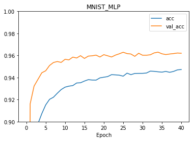
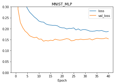
The plot method shows the value of various network metrics during training. The metrics loss and val_loss represent the value of the error (loss) function on the training and testing sets, respectively. Likewise, acc and val_acc represent the accuracy of the training and testing sets, respectively. The optional ymin and ymax keywords can be used to adjust the y-axis scale. For example:

net.plot(['acc', 'val_acc'], ymin=0.9, ymax=1)

net.plot(['loss', 'val_loss'], ymin=0, ymax=0.3)

After training, the index of the largest output value in response to an input image corresponds to the network’s digit classification. For example, test input #42 is shown below, along with the network’s response.

cx.view(net.dataset.test_inputs[42])

net.propagate(net.dataset.test_inputs[42])

[8.003044407733917e-12,
 4.14482776989189e-08,
 2.9302846087375656e-06,
 3.158657364110695e-06,
 0.9854525327682495,
 3.7257711937854765e-06,
 1.7312998257246193e-10,
 0.00046544571523554623,
 3.208596410786413e-07,
 0.014071854762732983]

cx.argmax(net.propagate(net.dataset.test_inputs[42]))

4

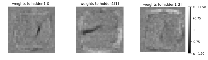
Examining the weights into the same three hidden units as before shows that these units have learned to respond in different ways to different parts of the input image.

net.plot_layer_weights('hidden1', units=[0,1,2], vshape=(28,28), wrange=(-1.5, 1.5))

3.3.2. A Convolutional Network for MNIST Classification

Convolutional neural networks (CNNs) are loosely inspired by the neurobiology of the visual system. The key idea is that each unit in a convolutional layer receives connections from a limited number of units in the previous layer (which can be thought of as the unit’s “visual field”), and these connections are arranged in a two-dimensional topology to take advantage of spatial information. Each convolutional layer specifies a number of independent features to be learned, along with the N × N size of the visual field (also called the kernel size). The units responsible for learning a feature share connections across the entire convolutional layer, which often leads to far fewer network parameters compared to a network with fully-connected layers.

Another type of layer common to CNNs is the pooling layer, which reduces the amount of information flowing through the network by the process of subsampling. Each pooling unit receives input from a limited number of units in the previous layer, and then applies some function (like maximum or average) to these inputs. The overall effect is to produce a coarser-grained version of the information from the previous layer, which makes the network less sensitive to small variations in position.

We will define a CNN for MNIST classification using two convolutional layers with 5 × 5 kernels, each followed by a pooling layer with 2 × 2 kernels that compute the maximum of their inputs. The first convolutional layer will learn 16 relatively low-level features, whereas the second will learn 32 higher-level features. These features will then feed into a hidden layer (after being flattened), followed by an output classification layer using Softmax.

cnn = cx.Network("MNIST_CNN")

cnn.add(cx.Layer("input", (28,28,1), colormap="gray"),
        cx.Conv2DLayer("conv2D_1", 16, (5,5), activation="relu", dropout=0.2),
        cx.MaxPool2DLayer("maxpool1", (2,2)),
        cx.Conv2DLayer("conv2D_2", 32, (5,5), activation="relu", dropout=0.2),
        cx.MaxPool2DLayer("maxpool2", (2,2)),
        cx.FlattenLayer("flat"),
        cx.Layer("hidden", 30, activation='relu'),
        cx.Layer("output", 10, activation='softmax'))

cnn.connect()

cnn.dataset.get("MNIST")
cnn.dataset.split(10000)
cnn.dataset.summary()

_________________________________________________________________
MNIST:
Patterns    Shape                 Range
=================================================================
inputs      (28, 28, 1)           (0.0, 1.0)
targets     (10,)                 (0.0, 1.0)
=================================================================
Total patterns: 70000
   Training patterns: 60000
   Testing patterns: 10000
_________________________________________________________________

cnn.compile(error='categorical_crossentropy', optimizer='rmsprop')
cnn.summary()

_________________________________________________________________
Layer (type)                 Output Shape              Param #
=================================================================
input (InputLayer)           (None, 28, 28, 1)         0
_________________________________________________________________
conv2D_1 (Conv2D)            (None, 24, 24, 16)        416
_________________________________________________________________
dropout_3 (Dropout)          (None, 24, 24, 16)        0
_________________________________________________________________
maxpool1 (MaxPooling2D)      (None, 12, 12, 16)        0
_________________________________________________________________
conv2D_2 (Conv2D)            (None, 8, 8, 32)          12832
_________________________________________________________________
dropout_4 (Dropout)          (None, 8, 8, 32)          0
_________________________________________________________________
maxpool2 (MaxPooling2D)      (None, 4, 4, 32)          0
_________________________________________________________________
flat (Flatten)               (None, 512)               0
_________________________________________________________________
hidden (Dense)               (None, 30)                15390
_________________________________________________________________
output (Dense)               (None, 10)                310
=================================================================
Total params: 28,948
Trainable params: 28,948
Non-trainable params: 0
_________________________________________________________________

cnn.dashboard()

cnn.train(epochs=5, batch_size=128)

========================================================
       |  Training |  Training |  Validate |  Validate
Epochs |     Error |  Accuracy |     Error |  Accuracy
------ | --------- | --------- | --------- | ---------
#    5 |   0.03536 |   0.98902 |   0.03667 |   0.98880