3.9. Plotting in 3D
This notebook demonstrates plotting 3D data in Conx.
In [1]:
import conx as cx
Using TensorFlow backend.
Conx, version 3.6.0
In [2]:
net = cx.Network("XOR", 2, 5, 1, activation="tanh")
In [3]:
net.picture()
Out[3]:
In [4]:
net.compile(error="mse", optimizer="sgd")
In [5]:
net.propagate([-.5, .5])
Out[5]:
[0.04958111792802811]
In [6]:
net.summary()
_________________________________________________________________
Layer (type)                 Output Shape              Param #
=================================================================
input (InputLayer)           (None, 2)                 0
_________________________________________________________________
hidden (Dense)               (None, 5)                 15
_________________________________________________________________
output (Dense)               (None, 1)                 6
=================================================================
Total params: 21
Trainable params: 21
Non-trainable params: 0
_________________________________________________________________
In [8]:
net.reset()
In [9]:
net.dataset.append([-1, -1], [-1])
net.dataset.append([-1, +1], [+1])
net.dataset.append([+1, -1], [+1])
net.dataset.append([+1, +1], [-1])
In [10]:
dash = net.dashboard()
dash
In [11]:
net.train(10000, accuracy=1.0, tolerance=.1, plot=True, report_rate=200)

========================================================
       |  Training |  Training
Epochs |     Error |  Accuracy
------ | --------- | ---------
# 2257 |   0.00859 |   1.00000
In [12]:
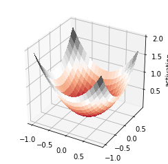
cx.plot3D(lambda x,y: x ** 2 + y ** 2, (-1,1,.1), (-1,1,.1), label="Label",
          zlabel="activation", linewidth=0, colormap="RdGy", mode="surface")
In [13]:
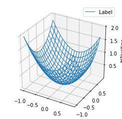
cx.plot3D(lambda x,y: x ** 2 + y ** 2, (-1,1,.1), (-1,1,.1), label="Label",
          zlabel="activation", linewidth=1, colormap="RdGy", mode="wireframe")
In [14]:
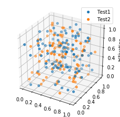
import random
points1 = []
for i in range(100):
    points1.append([random.random(), random.random(), random.random()])
points2 = []
for i in range(100):
    points2.append([random.random(), random.random(), random.random()])

cx.plot3D([["Test1", points1], ["Test2", points2]], zlabel="activation", mode="scatter")
In [15]:
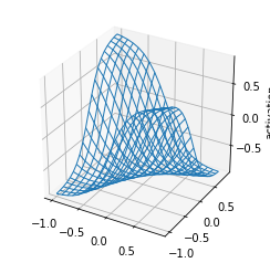
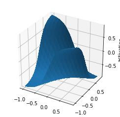
cx.plot3D(lambda x,y: net.propagate([x,y])[0], (-1, 1, .1), (-1, 1, .1),
          zlabel="activation",
          mode="surface")
In [16]:
cx.plot3D(lambda x,y: net.propagate([x,y])[0], (-1, 1, .1), (-1, 1, .1),
          zlabel="activation",
          mode="wireframe", linewidth=1)