3.24. Utilities
This notebook demonstrates the Conx utility functions.
First, we import the conx library:
In [1]:
import conx as cx
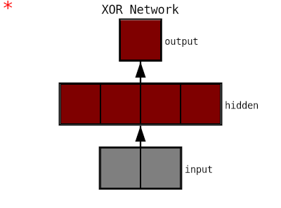
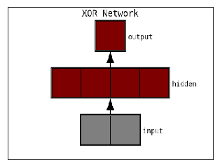
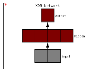
net = cx.Network("XOR Network", 2, 4, 1, activation="sigmoid")
Using TensorFlow backend.
Conx, version 3.6.1
3.24.1. Images
array_to_image(array, scale=1.0, shape=None)
In [2]:
r, g, b = 0, 0, 1
array = [[[r,g,b] for col in range(400)] for row in range(200)]
image = cx.array_to_image(array)
image
Out[2]:

image_to_array(image)
In [3]:
cx.shape(cx.image_to_array(image))
Out[3]:
(200, 400, 3)
In [4]:
cx.image_to_array(image)[0][0]
Out[4]:
[0.0, 0.0, 1.0]
svg_to_image(svg, background=(255, 255, 255, 255))
In [5]:
svg = net._repr_svg_()
image = cx.svg_to_image(svg)
image
Out[5]:
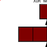
crop_image(image, x1, y1, x2, y2)
In [6]:
cx.crop_image(image, 10, 10, 200, 200)
Out[6]:
3.24.2. Plotting
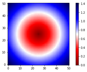
heatmap()
In [27]:
import math
def function(x, y):
    return math.sqrt(x ** 2 + y ** 2)
hm = cx.heatmap(function,  in_range=(-1,1))
hm
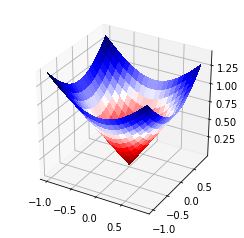
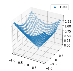
plot3D()
In [24]:
cx.plot3D(function, x_range=(-1,1,.1), y_range=(-1,1,.1), colormap=cx.get_colormap(), mode="surface")
In [23]:
cx.plot3D([["Data", [(x,y,function(x,y)) for x in cx.frange(-1,1,.1) for y in cx.frange(-1,1,.1)]]],
          mode="scatter")
In [28]:
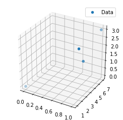
cx.plot3D([["Data", [(0,1,0), (1,2,3), (1,3,2), (1,7,3)]]], mode="scatter")
plot()
In [19]:
symbols = {"Apples": "x", "Bananas": "o-"}
In [24]:
cx.plot([["Apples", [3, 5, 7]],
         ["Bananas",[4, 2, 8]]],
        symbols=symbols)
Out[24]:

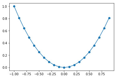
plot_f()
In [30]:
cx.plot_f(lambda x: x ** 2)
scatter()
In [23]:
cx.scatter([["Apples", [(3,3), (1,5), (7,4)]],
            ["Bananas",[(3,4), (5,4), (8,2)]]],
          symbols=symbols)
Out[23]:

3.24.3. Console Utilities
show(item, title, background=(255, 255, 255, 255))
In [10]:
cx.view(net)
In [11]:
cx.view(net, title="My Title", background=(0, 128, 255, 255))

view_image(image, title)
In [12]:
cx.view_image(image)
show_svg(svg, title, background=(255, 255, 255, 255))
In [13]:
cx.view_svg(net._repr_svg_())

3.24.4. Miscellaneous
movie(…)
In [ ]:
cx.movie()
reshape(matrix, new_shape)
In [42]:
m = [[1, 2, 3], [4, 5, 6]]
print(cx.shape(m))
m = cx.reshape(m, (3, 2))
print(cx.shape(m))
m
(2, 3)
(3, 2)
Out[42]:
[[1, 2], [3, 4], [5, 6]]
onehot(i, width)
In [43]:
cx.onehot(5, 10)
Out[43]:
[0, 0, 0, 0, 0, 1, 0, 0, 0, 0]
shape(item)
In [45]:
cx.shape([[3], [4]])
Out[45]:
(2, 1)
argmax(seq)
In [50]:
cx.argmax([1, 2, 3, 4, 8, 4, 3, 2, 1])
Out[50]:
4
argmin(seq)
In [49]:
cx.argmin([7, 3, 2, 5, 1, 7])
Out[49]:
4
maximum(seq)
In [52]:
cx.maximum([8, 4, 2, 6, 8])
Out[52]:
8
minimum(seq)
In [53]:
cx.minimum([8, 4, 2, 6, 8])
Out[53]:
2
binary(i, width)
In [56]:
cx.binary(23, 10)
Out[56]:
[0, 0, 0, 0, 0, 1, 0, 1, 1, 1]
choice(seq=None, p=None)
In [57]:
cx.choice("abcdefg", p=[0, .1, .2, .4, .1, .2, 0])
Out[57]:
'f'
download(url, directory=”./”, force=False, unzip=True)
In [61]:
from IPython.display import Image
cx.download("https://github.com/Calysto/conx-notebooks/raw/master/calysto.gif")
Image(data="calysto.gif")
Using cached https://github.com/Calysto/conx-notebooks/raw/master/calysto.gif as './calysto.gif'.
Out[61]:
<IPython.core.display.Image object>
frange(start, stop=None, step=1.0)
In [62]:
cx.frange(-1, 1, .25)
Out[62]:
[-1.0, -0.75, -0.5, -0.25, 0.0, 0.25, 0.5, 0.75]
get_device()
In [39]:
cx.get_device()
Out[39]:
'cpu'
3.24.5. Colormaps
get_colormap()
In [31]:
cx.get_colormap()
Out[31]:
'seismic_r'
get_error_colormap()
In [32]:
cx.get_error_colormap()
Out[32]:
'seismic_r'
In [35]:
cx.AVAILABLE_COLORMAPS[:10]
Out[35]:
['Accent',
 'Accent_r',
 'Blues',
 'Blues_r',
 'BrBG',
 'BrBG_r',
 'BuGn',
 'BuGn_r',
 'BuPu',
 'BuPu_r']
set_colormap()
In [37]:
cx.set_colormap('Accent')
set_error_colormap(s)
In [36]:
cx.set_error_colormap("gray")
3.24.6. Under Development
import_keras_model(model, network_name)